# install.packages("tidymodels")
# install.packages("xgboost")
# install.packages("vip")
# install.packages("pdp")

library(tidymodels)
library(vip)
library(pdp)
library(xgboost)
tidymodels_prefer() # resolves MASS::select() vs dplyr::select(), etc.Boosting
Boosting — with tidymodels
We will replicate ISLR Lab 8.3.4 — The original lab uses the gbm package to fit boosted regression trees on the Boston housing data, predicting medv (median home value). parsnip has no native “gbm” engine, so we use boost_tree() with the “xgboost” engine — the standard tidymodels equivalent for gradient boosting. Argument mapping used throughout:
- gbm argument -> parsnip / boost_tree argument
- n.trees -> trees
- interaction.depth -> tree_depth
- shrinkage -> learn_rate
- distribution=“gaussian” -> set_mode(“regression”)
Packages needed: tidymodels, xgboost, MASS (for the original Boston data), vip (variable importance), pdp (partial dependence, as in the book)
1. Load the data
MASS::Boston is the original dataset used in the 1st-edition ISLR lab.
data(Boston, package = "MASS")
boston <- as_tibble(Boston)

glimpse(boston)
Rows: 506
Columns: 14
$ crim <dbl> 0.00632, 0.02731, 0.02729, 0.03237, 0.06905, 0.02985, 0.08829,…
$ zn <dbl> 18.0, 0.0, 0.0, 0.0, 0.0, 0.0, 12.5, 12.5, 12.5, 12.5, 12.5, 1…
$ indus <dbl> 2.31, 7.07, 7.07, 2.18, 2.18, 2.18, 7.87, 7.87, 7.87, 7.87, 7.…
$ chas <int> 0, 0, 0, 0, 0, 0, 0, 0, 0, 0, 0, 0, 0, 0, 0, 0, 0, 0, 0, 0, 0,…
$ nox <dbl> 0.538, 0.469, 0.469, 0.458, 0.458, 0.458, 0.524, 0.524, 0.524,…
$ rm <dbl> 6.575, 6.421, 7.185, 6.998, 7.147, 6.430, 6.012, 6.172, 5.631,…
$ age <dbl> 65.2, 78.9, 61.1, 45.8, 54.2, 58.7, 66.6, 96.1, 100.0, 85.9, 9…
$ dis <dbl> 4.0900, 4.9671, 4.9671, 6.0622, 6.0622, 6.0622, 5.5605, 5.9505…
$ rad <int> 1, 2, 2, 3, 3, 3, 5, 5, 5, 5, 5, 5, 5, 4, 4, 4, 4, 4, 4, 4, 4,…
$ tax <dbl> 296, 242, 242, 222, 222, 222, 311, 311, 311, 311, 311, 311, 31…
$ ptratio <dbl> 15.3, 17.8, 17.8, 18.7, 18.7, 18.7, 15.2, 15.2, 15.2, 15.2, 15…
$ black <dbl> 396.90, 396.90, 392.83, 394.63, 396.90, 394.12, 395.60, 396.90…
$ lstat <dbl> 4.98, 9.14, 4.03, 2.94, 5.33, 5.21, 12.43, 19.15, 29.93, 17.10…
$ medv <dbl> 24.0, 21.6, 34.7, 33.4, 36.2, 28.7, 22.9, 27.1, 16.5, 18.9, 15…2. Recreate the book’s exact train/test split
Note
- The lab uses: set.seed(1); train <- sample(1:nrow(Boston), nrow(Boston)/2)
- We reproduce that exactly, then wrap the indices into an rsample split
- object with make_splits() so the rest of the pipeline can use standard
- tidymodels verbs (training(), testing()).
set.seed(1)
train_idx <- sample(seq_len(nrow(boston)), size = nrow(boston) / 2)
test_idx <- setdiff(seq_len(nrow(boston)), train_idx)

boston_split <- make_splits(
  x    = list(analysis = train_idx, assessment = test_idx),
  data = boston
)
boston_train <- training(boston_split)
boston_test <- testing(boston_split)

nrow(boston_train) # matches length(train) == 253 in the book
[1] 2533. Preprocessing recipe
Boosted trees need no dummy-coding, centering, or scaling. The recipe here is effectively a pass-through, included mainly for pipeline consistency.
boston_rec <- recipe(medv ~ ., data = boston_train)4. Model specification #1
We match the book’s first gbm() call:
Book:
- set.seed(1)
- boost.boston <- gbm(medv ~ ., data = Boston[train, ], distribution = “gaussian”, n.trees = 5000, interaction.depth = 4)
- (shrinkage unspecified -> gbm’s default of 0.001)
boost_spec_default_shrinkage <-
  boost_tree(
    trees      = 5000,
    tree_depth = 4,
    learn_rate = 0.001
  ) |>
  set_engine("xgboost") |>
  set_mode("regression")
boston_wflow_1 <-
  workflow() |>
  add_recipe(boston_rec) |>
  add_model(boost_spec_default_shrinkage)

set.seed(1)
boston_fit_1 <- fit(boston_wflow_1, data = boston_train)
5. Variable importance (“relative influence” in the book’s summary())
boston_fit_1 |>
  extract_fit_parsnip() |>
  vip(num_features = 13) +
  labs(title = "Relative Influence of Predictors (Boosted Trees)")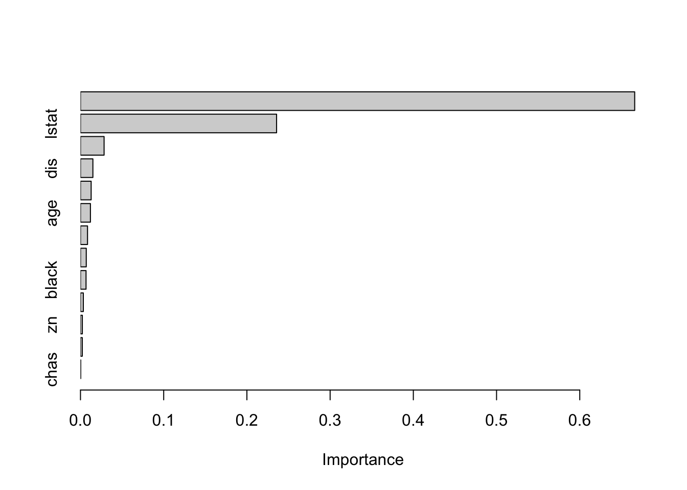
NULL6. Partial dependence plots for lstat and rm
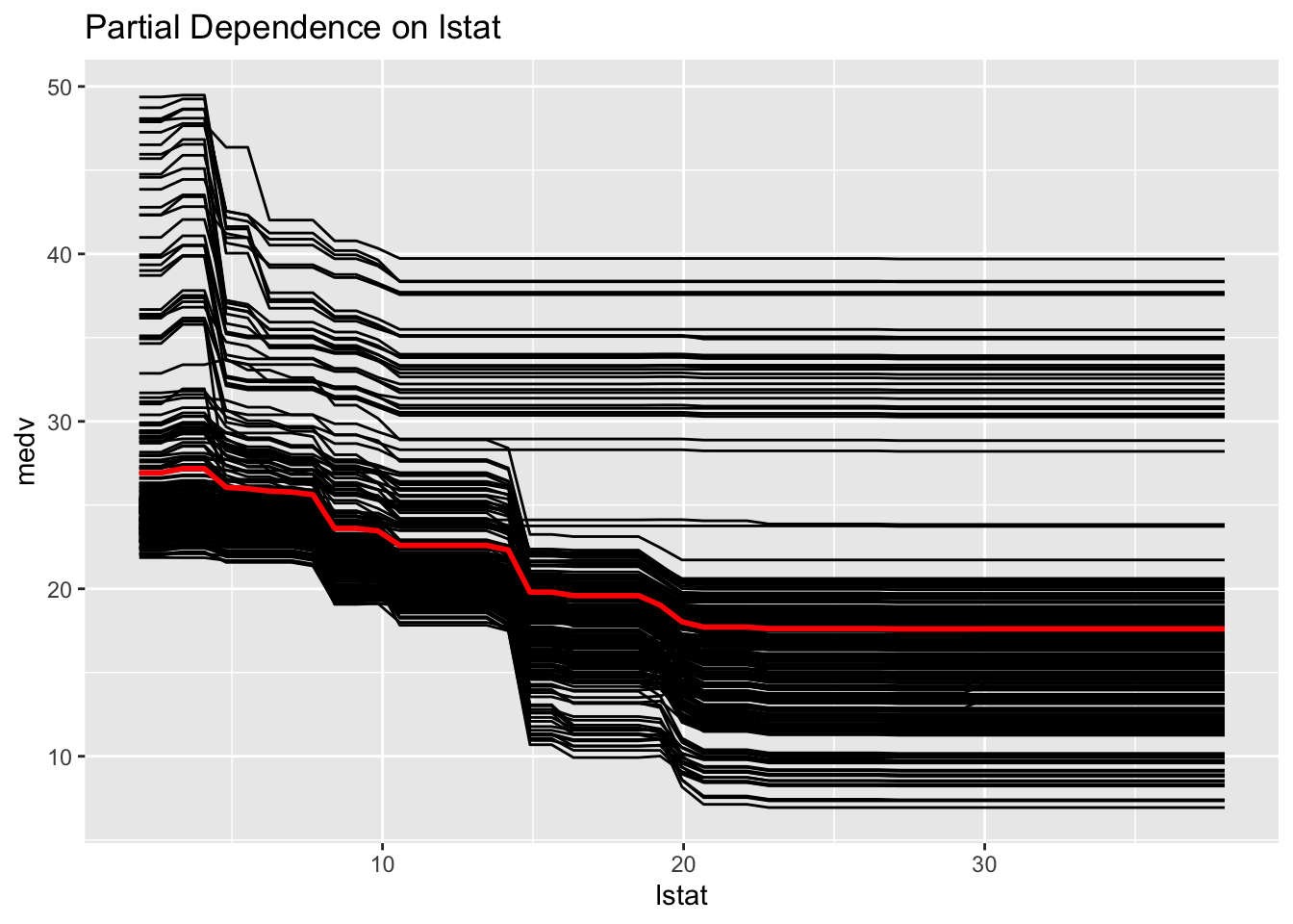
Book:
- plot(boost.boston, i = “lstat”)
- plot(boost.boston, i = “rm”)
- pdp::partial() works directly on the fitted workflow.
pdp_rm <- pdp::partial(
  boston_fit_1,
  pred.var = "rm",
  train    = boston_train,
  type     = "regression",
  pred.fun = pred_wrapper
)
autoplot(pdp_rm) +
  labs(title = "Partial Dependence on rm", y = "medv")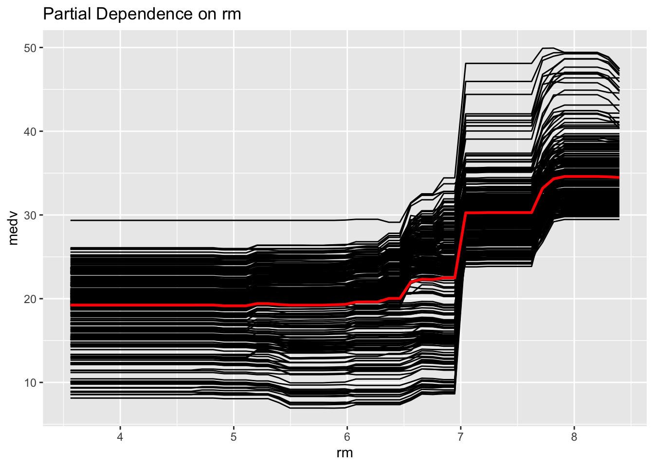
7. Predict on the test set and compute test MSE
Note
Book: - yhat.boost <- predict(boost.boston, newdata = Boston[-train, ], n.trees = 5000) - mean((yhat.boost - boston.test)^2)
[1] 22.06423# Equivalent yardstick metrics, for reference
boston_preds_1 |> rmse(truth = medv, estimate = .pred)boston_preds_1 |> rsq(truth = medv, estimate = .pred)8. Model specification #2 — higher shrinkage, as in the book’s comparison
Note
Book:
- boost.boston <- gbm(medv ~ ., data = Boston[train, ],
distribution = "gaussian", n.trees = 5000,interaction.depth = 4, shrinkage = 0.2, verbose = F)- yhat.boost <- predict(boost.boston, newdata = Boston[-train, ], n.trees = 5000)
- mean((yhat.boost - boston.test)^2) # book reports ~15.07 (lower/better)
boost_spec_shrink_0.2 <-
  boost_tree(
    trees      = 5000,
    tree_depth = 4,
    learn_rate = 0.2
  ) |>
  set_engine("xgboost") |>
  set_mode("regression")

boston_wflow_2 <-
  workflow() |>
  add_recipe(boston_rec) |>
  add_model(boost_spec_shrink_0.2)
set.seed(1)
boston_fit_2 <- fit(boston_wflow_2, data = boston_train)

boston_preds_2 <- predict(boston_fit_2, new_data = boston_test) |>
  bind_cols(boston_test |> select(medv))

test_mse_2 <- mean((boston_preds_2$.pred - boston_preds_2$medv)^2)
test_mse_2
[1] 21.64269. Compare the two shrinkage values, as the book does
Notes on fidelity to the original lab
-
xgboostandgbmimplement gradient boosting slightly differently - (e.g. regularization terms, split-finding algorithm), so exact MSE
- values won’t match the book number-for-number, but the qualitative
- result should replicate: a higher learn_rate / shrinkage noticeably
- changes test MSE, and lstat and rm emerge as the most influential
- predictors, matching the book’s summary() output.
- If an exact match to gbm’s algorithm is important, the
bonsaipackage
- If an exact match to gbm’s algorithm is important, the
- also offers a “lightgbm” engine for
boost_tree(), or gbm can be called - directly as in the original lab; xgboost is used here as it’s the
- default, most widely supported boosting engine in parsnip.