# install.packages("tidymodels")
# install.packages("tidyclust")
# install.packages("ISLR")

library(tidymodels)
library(tidyclust)
library(ISLR)
tidymodels_prefer()K-means Clustering
K-Means Clustering with tidymodels (tidyclust) — NCI60 Dataset
- NCI60 (from ISLR) contains gene expression measurements for 6,830 genes across 64 cancer cell lines. = It has no outcome variable — it’s classic unsupervised learning territory, used in ISLR’s clustering lab.
- We cluster the cell lines by gene expression and compare the resulting clusters against the known cancer-type labels (which are NOT used in clustering, only for post-hoc evaluation).
tidymodels itself doesn’t include clustering verbs — clustering support lives in the tidyclust extension package, which mirrors parsnip/workflows conventions (k_means(), set_engine(), workflow(), tune_cluster(), etc.).
Packages needed: tidymodels, tidyclust, ISLR (for NCI60), factoextra (optional, for PCA visualization)
1. Load and prepare the data
[1] 64 6830table(nci_labs) # the cancer types we'll compare clusters againstnci_labs
BREAST CNS COLON K562A-repro K562B-repro LEUKEMIA
7 5 7 1 1 6
MCF7A-repro MCF7D-repro MELANOMA NSCLC OVARIAN PROSTATE
1 1 8 9 6 2
RENAL UNKNOWN
9 1 2. Preprocessing recipe
Gene expression columns are already on a common (microarray-normalized) scale, but standardizing each gene to mean 0 / sd 1 is still standard practice before k-means, since it’s a distance-based method and any gene with naturally larger variance would otherwise dominate the Euclidean distance calculation. Zero-variance genes (if any) are dropped.
nci_rec <-
  recipe(~., data = nci_data) |>
  step_zv(all_predictors()) |>
  step_normalize(all_predictors()) |>
  step_pca(all_predictors(), num_comp = 10) # reduce 6,830 genes -> 10 PCs
3. Model specification (tunable number of clusters)
kmeans_spec <-
  k_means(num_clusters = tune()) |>
  set_engine("stats")
4. Workflow: bundle recipe + model
nci_wflow <-
  workflow() |>
  add_recipe(nci_rec) |>
  add_model(kmeans_spec)
5. Choose k via resampling + cluster metrics
With only 64 observations, we use bootstrap resamples rather than v-fold CV (there’s no outcome to “predict,” so resampling here is purely to get a stability-aware estimate of cluster quality across k).
set.seed(123)
nci_boots <- bootstraps(nci_data, times = 3)

k_grid <- tibble(num_clusters = c(2, 4, 6))

nci_tune_results <-
  nci_wflow |>
  tune_cluster(
    resamples = nci_boots,
    grid      = k_grid,
    metrics   = cluster_metric_set(sse_within_total, sse_total, sse_ratio),
    # control   = control_cluster(verbose = TRUE)
  )

# "Elbow plot": within-cluster SSE ratio vs. number of clusters
nci_tune_results |>
  collect_metrics() |>
  filter(.metric == "sse_ratio") |>
  ggplot(aes(x = num_clusters, y = mean)) +
  geom_line() +
  geom_point() +
  scale_x_continuous(breaks = 2:10) +
  labs(
    title = "Elbow Plot — Choosing k for NCI60 K-Means",
    x = "Number of clusters (k)",
    y = "Mean SSE ratio (within-cluster SSE / total SSE)"
  ) +
  theme_minimal()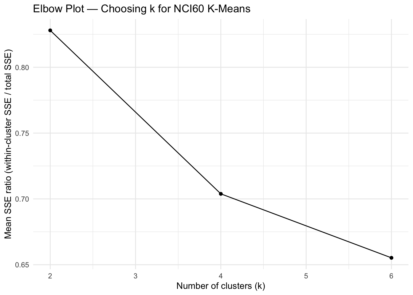
show_best(nci_tune_results, metric = "sse_ratio", n = 5)6. Finalize the workflow with a chosen k
- Pick k using the elbow plot above (where adding another cluster stops producing a meaningful drop in SSE ratio). - ISLR’s own clustering lab settles on 4 clusters for NCI60 as a reasonable, interpretable choice — used here directly, but feel free to substitute the elbow-selected value.
final_k <- 4

final_wflow <- nci_wflow |>
  finalize_workflow_tidyclust(tibble(num_clusters = final_k))
7. Fit the final k-means model
set.seed(456)
nci_fit <- fit(final_wflow, data = nci_data)
# Cluster centroids (mean expression profile per cluster, in normalized units)
nci_fit |> extract_centroids()
8. Extract cluster assignments and compare to known cancer types
cluster_assignments <- extract_cluster_assignment(nci_fit)

nci_results <- tibble(
  cell_line     = seq_along(nci_labs),
  cancer_type   = nci_labs,
  cluster       = cluster_assignments$.cluster
)

# Cross-tabulate clusters against known cancer types (as in the ISLR lab)
nci_results |>
  count(cluster, cancer_type) |>
  pivot_wider(names_from = cancer_type, values_from = n, values_fill = 0)
9. Evaluate overall cluster quality
nci_fit |> sse_within_total()nci_fit |> sse_ratio()# Silhouette needs the (preprocessed) data used for clustering
nci_baked <- bake(extract_recipe(nci_fit), new_data = nci_data)
nci_fit |> silhouette_avg(nci_baked)Error in `hardhat::forge()`:
! The required columns "1", "2", "3", "4", "5", "6", "7", "8", "9",
"10", "11", "12", "13", "14", "15", "16", "17", "18", …, "6829", and "6830"
are missing.10. Visualize clusters on the first two principal components
As in the ISLR lab, plotting on PCA scores gives a 2D view of a fundamentally high-dimensional (6,830-gene) clustering result.
nci_pca <- prcomp(nci_baked, scale. = FALSE) # already standardized upstream

pca_scores <- as_tibble(nci_pca$x[, 1:2]) |>
  mutate(
    cluster     = factor(cluster_assignments$.cluster),
    cancer_type = nci_labs
  )

ggplot(pca_scores, aes(x = PC1, y = PC2, color = cluster)) +
  geom_point(size = 2) +
  labs(
    title = "NCI60 Cell Lines Clustered by Gene Expression (k = 4)",
    subtitle = "Projected onto the first two principal components",
    x = "PC1", y = "PC2", color = "Cluster"
  ) +
  theme_minimal()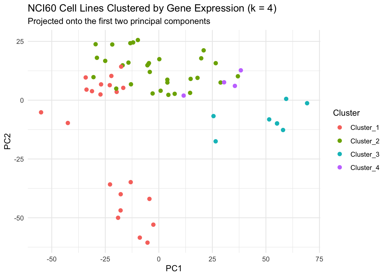
11. (Optional) Extract the final fitted workflow for reuse
# saveRDS(nci_fit, "nci60_kmeans_workflow.rds")

# Example: assign new/unseen samples to the nearest existing cluster
# predict(nci_fit, new_data = some_new_data)