library(tidymodels)
tidymodels_prefer() # resolves common function-name conflicts (e.g. select())Linear Regression with tidymodels
Linear Regression with tidymodels — AMES Housing Dataset
Packages needed: tidymodels (includes rsample, recipes, parsnip, workflows, tune, yardstick, etc.), and the AMES data itself, which ships in themodeldata package (a tidymodels package) as ames.
1. Load and inspect the data
Rows: 2,930
Columns: 74
$ MS_SubClass        <fct> One_Story_1946_and_Newer_All_Styles, One_Story_1946…
$ MS_Zoning          <fct> Residential_Low_Density, Residential_High_Density, …
$ Lot_Frontage       <dbl> 141, 80, 81, 93, 74, 78, 41, 43, 39, 60, 75, 0, 63,…
$ Lot_Area           <int> 31770, 11622, 14267, 11160, 13830, 9978, 4920, 5005…
$ Street             <fct> Pave, Pave, Pave, Pave, Pave, Pave, Pave, Pave, Pav…
$ Alley              <fct> No_Alley_Access, No_Alley_Access, No_Alley_Access, …
$ Lot_Shape          <fct> Slightly_Irregular, Regular, Slightly_Irregular, Re…
$ Land_Contour       <fct> Lvl, Lvl, Lvl, Lvl, Lvl, Lvl, Lvl, HLS, Lvl, Lvl, L…
$ Utilities          <fct> AllPub, AllPub, AllPub, AllPub, AllPub, AllPub, All…
$ Lot_Config         <fct> Corner, Inside, Corner, Corner, Inside, Inside, Ins…
$ Land_Slope         <fct> Gtl, Gtl, Gtl, Gtl, Gtl, Gtl, Gtl, Gtl, Gtl, Gtl, G…
$ Neighborhood       <fct> North_Ames, North_Ames, North_Ames, North_Ames, Gil…
$ Condition_1        <fct> Norm, Feedr, Norm, Norm, Norm, Norm, Norm, Norm, No…
$ Condition_2        <fct> Norm, Norm, Norm, Norm, Norm, Norm, Norm, Norm, Nor…
$ Bldg_Type          <fct> OneFam, OneFam, OneFam, OneFam, OneFam, OneFam, Twn…
$ House_Style        <fct> One_Story, One_Story, One_Story, One_Story, Two_Sto…
$ Overall_Cond       <fct> Average, Above_Average, Above_Average, Average, Ave…
$ Year_Built         <int> 1960, 1961, 1958, 1968, 1997, 1998, 2001, 1992, 199…
$ Year_Remod_Add     <int> 1960, 1961, 1958, 1968, 1998, 1998, 2001, 1992, 199…
$ Roof_Style         <fct> Hip, Gable, Hip, Hip, Gable, Gable, Gable, Gable, G…
$ Roof_Matl          <fct> CompShg, CompShg, CompShg, CompShg, CompShg, CompSh…
$ Exterior_1st       <fct> BrkFace, VinylSd, Wd Sdng, BrkFace, VinylSd, VinylS…
$ Exterior_2nd       <fct> Plywood, VinylSd, Wd Sdng, BrkFace, VinylSd, VinylS…
$ Mas_Vnr_Type       <fct> Stone, None, BrkFace, None, None, BrkFace, None, No…
$ Mas_Vnr_Area       <dbl> 112, 0, 108, 0, 0, 20, 0, 0, 0, 0, 0, 0, 0, 0, 0, 6…
$ Exter_Cond         <fct> Typical, Typical, Typical, Typical, Typical, Typica…
$ Foundation         <fct> CBlock, CBlock, CBlock, CBlock, PConc, PConc, PConc…
$ Bsmt_Cond          <fct> Good, Typical, Typical, Typical, Typical, Typical, …
$ Bsmt_Exposure      <fct> Gd, No, No, No, No, No, Mn, No, No, No, No, No, No,…
$ BsmtFin_Type_1     <fct> BLQ, Rec, ALQ, ALQ, GLQ, GLQ, GLQ, ALQ, GLQ, Unf, U…
$ BsmtFin_SF_1       <dbl> 2, 6, 1, 1, 3, 3, 3, 1, 3, 7, 7, 1, 7, 3, 3, 1, 3, …
$ BsmtFin_Type_2     <fct> Unf, LwQ, Unf, Unf, Unf, Unf, Unf, Unf, Unf, Unf, U…
$ BsmtFin_SF_2       <dbl> 0, 144, 0, 0, 0, 0, 0, 0, 0, 0, 0, 0, 0, 0, 1120, 0…
$ Bsmt_Unf_SF        <dbl> 441, 270, 406, 1045, 137, 324, 722, 1017, 415, 994,…
$ Total_Bsmt_SF      <dbl> 1080, 882, 1329, 2110, 928, 926, 1338, 1280, 1595, …
$ Heating            <fct> GasA, GasA, GasA, GasA, GasA, GasA, GasA, GasA, Gas…
$ Heating_QC         <fct> Fair, Typical, Typical, Excellent, Good, Excellent,…
$ Central_Air        <fct> Y, Y, Y, Y, Y, Y, Y, Y, Y, Y, Y, Y, Y, Y, Y, Y, Y, …
$ Electrical         <fct> SBrkr, SBrkr, SBrkr, SBrkr, SBrkr, SBrkr, SBrkr, SB…
$ First_Flr_SF       <int> 1656, 896, 1329, 2110, 928, 926, 1338, 1280, 1616, …
$ Second_Flr_SF      <int> 0, 0, 0, 0, 701, 678, 0, 0, 0, 776, 892, 0, 676, 0,…
$ Gr_Liv_Area        <int> 1656, 896, 1329, 2110, 1629, 1604, 1338, 1280, 1616…
$ Bsmt_Full_Bath     <dbl> 1, 0, 0, 1, 0, 0, 1, 0, 1, 0, 0, 1, 0, 1, 1, 1, 0, …
$ Bsmt_Half_Bath     <dbl> 0, 0, 0, 0, 0, 0, 0, 0, 0, 0, 0, 0, 0, 0, 0, 0, 0, …
$ Full_Bath          <int> 1, 1, 1, 2, 2, 2, 2, 2, 2, 2, 2, 2, 2, 1, 1, 3, 2, …
$ Half_Bath          <int> 0, 0, 1, 1, 1, 1, 0, 0, 0, 1, 1, 0, 1, 1, 1, 1, 0, …
$ Bedroom_AbvGr      <int> 3, 2, 3, 3, 3, 3, 2, 2, 2, 3, 3, 3, 3, 2, 1, 4, 4, …
$ Kitchen_AbvGr      <int> 1, 1, 1, 1, 1, 1, 1, 1, 1, 1, 1, 1, 1, 1, 1, 1, 1, …
$ TotRms_AbvGrd      <int> 7, 5, 6, 8, 6, 7, 6, 5, 5, 7, 7, 6, 7, 5, 4, 12, 8,…
$ Functional         <fct> Typ, Typ, Typ, Typ, Typ, Typ, Typ, Typ, Typ, Typ, T…
$ Fireplaces         <int> 2, 0, 0, 2, 1, 1, 0, 0, 1, 1, 1, 0, 1, 1, 0, 1, 0, …
$ Garage_Type        <fct> Attchd, Attchd, Attchd, Attchd, Attchd, Attchd, Att…
$ Garage_Finish      <fct> Fin, Unf, Unf, Fin, Fin, Fin, Fin, RFn, RFn, Fin, F…
$ Garage_Cars        <dbl> 2, 1, 1, 2, 2, 2, 2, 2, 2, 2, 2, 2, 2, 2, 2, 3, 2, …
$ Garage_Area        <dbl> 528, 730, 312, 522, 482, 470, 582, 506, 608, 442, 4…
$ Garage_Cond        <fct> Typical, Typical, Typical, Typical, Typical, Typica…
$ Paved_Drive        <fct> Partial_Pavement, Paved, Paved, Paved, Paved, Paved…
$ Wood_Deck_SF       <int> 210, 140, 393, 0, 212, 360, 0, 0, 237, 140, 157, 48…
$ Open_Porch_SF      <int> 62, 0, 36, 0, 34, 36, 0, 82, 152, 60, 84, 21, 75, 0…
$ Enclosed_Porch     <int> 0, 0, 0, 0, 0, 0, 170, 0, 0, 0, 0, 0, 0, 0, 0, 0, 0…
$ Three_season_porch <int> 0, 0, 0, 0, 0, 0, 0, 0, 0, 0, 0, 0, 0, 0, 0, 0, 0, …
$ Screen_Porch       <int> 0, 120, 0, 0, 0, 0, 0, 144, 0, 0, 0, 0, 0, 0, 140, …
$ Pool_Area          <int> 0, 0, 0, 0, 0, 0, 0, 0, 0, 0, 0, 0, 0, 0, 0, 0, 0, …
$ Pool_QC            <fct> No_Pool, No_Pool, No_Pool, No_Pool, No_Pool, No_Poo…
$ Fence              <fct> No_Fence, Minimum_Privacy, No_Fence, No_Fence, Mini…
$ Misc_Feature       <fct> None, None, Gar2, None, None, None, None, None, Non…
$ Misc_Val           <int> 0, 0, 12500, 0, 0, 0, 0, 0, 0, 0, 0, 500, 0, 0, 0, …
$ Mo_Sold            <int> 5, 6, 6, 4, 3, 6, 4, 1, 3, 6, 4, 3, 5, 2, 6, 6, 6, …
$ Year_Sold          <int> 2010, 2010, 2010, 2010, 2010, 2010, 2010, 2010, 201…
$ Sale_Type          <fct> WD , WD , WD , WD , WD , WD , WD , WD , WD , WD , W…
$ Sale_Condition     <fct> Normal, Normal, Normal, Normal, Normal, Normal, Nor…
$ Sale_Price         <dbl> 5.332438, 5.021189, 5.235528, 5.387390, 5.278525, 5…
$ Longitude          <dbl> -93.61975, -93.61976, -93.61939, -93.61732, -93.638…
$ Latitude           <dbl> 42.05403, 42.05301, 42.05266, 42.05125, 42.06090, 4…
2. Split the data: train / test
set.seed(123)

ames_split <- initial_split(ames, prop = 0.80, strata = Sale_Price)
ames_train <- training(ames_split)
ames_test <- testing(ames_split)
3. Preprocessing recipe
We’ll predict Sale_Price from a handful of informative predictors: - living area, lot area, year built, overall condition/quality, neighborhood, and building type.
ames_rec <-
  recipe(
    Sale_Price ~ Gr_Liv_Area + Lot_Area + Year_Built +
      Overall_Cond + Neighborhood + Bldg_Type,
    data = ames_train
  ) |>
  # log-transform skewed numeric predictors
  step_log(Gr_Liv_Area, Lot_Area, base = 10) |>
  # collapse rare neighborhood levels into "other" before dummy-coding
  step_other(Neighborhood, threshold = 0.01) |>
  # create dummy variables for all nominal (factor/character) predictors
  step_dummy(all_nominal_predictors()) |>
  # drop any predictor columns that end up with zero variance
  step_zv(all_predictors()) |>
  # center and scale numeric predictors
  step_normalize(all_numeric_predictors())
4. Model specification
lm_spec <-
  linear_reg() |>
  set_engine("lm") |>
  set_mode("regression")
5. Workflow: bundle recipe + model
ames_wflow <-
  workflow() |>
  add_recipe(ames_rec) |>
  add_model(lm_spec)
6. Fit on the training data
ames_fit <- fit(ames_wflow, data = ames_train)

# Tidy view of coefficients
ames_fit |>
  extract_fit_parsnip() |>
  tidy() |>
  arrange(desc(abs(estimate)))
7. Evaluate with 10-fold cross-validation (on training data)
set.seed(456)
ames_folds <- vfold_cv(ames_train, v = 10, strata = Sale_Price)

ames_cv_results <-
  ames_wflow |>
  fit_resamples(
    resamples = ames_folds,
    metrics   = metric_set(rmse, rsq, mae),
    control   = control_resamples(save_pred = TRUE)
  )

collect_metrics(ames_cv_results)
8. Final fit on full training set + evaluation on the held-out test set
final_fit <- last_fit(
  ames_wflow,
  split   = ames_split,
  metrics = metric_set(rmse, rsq, mae)
)

# Test-set performance
collect_metrics(final_fit)
# Predictions vs. truth on the test set
test_predictions <- collect_predictions(final_fit)
head(test_predictions)9. Visualize predicted vs. actual (log10) sale price
ggplot(test_predictions, aes(x = Sale_Price, y = .pred)) +
  geom_point(alpha = 0.4) +
  geom_abline(intercept = 0, slope = 1, color = "red", linetype = "dashed") +
  coord_obs_pred() +
  labs(
    title = "Predicted vs. Actual Sale Price (log10 scale)",
    x = "Actual log10(Sale_Price)",
    y = "Predicted log10(Sale_Price)"
  ) +
  theme_minimal()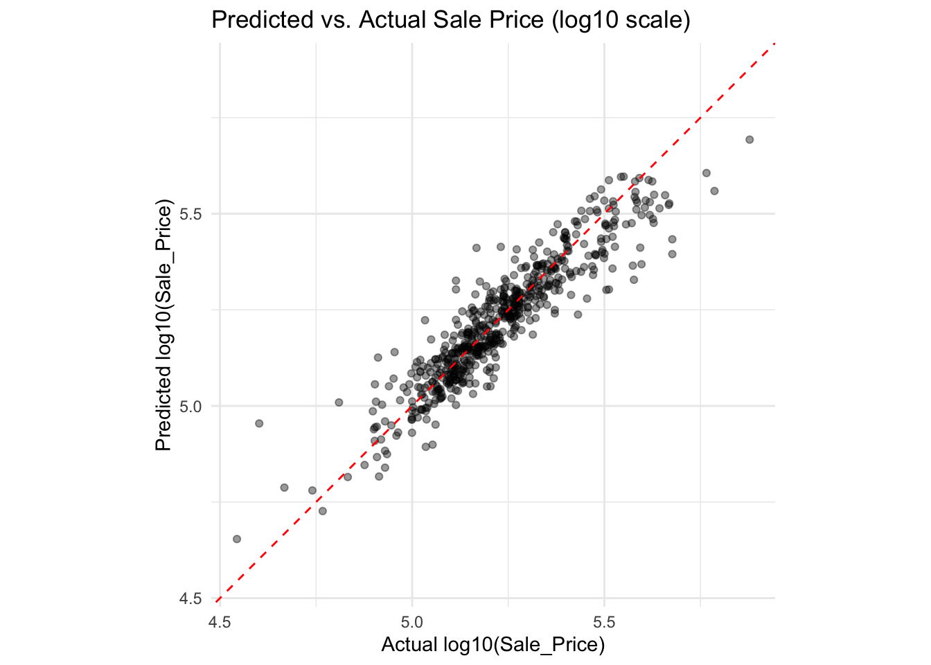
10.(Optional) Extract the final fitted workflow for reuse / deployment
final_wflow_fit <- extract_workflow(final_fit)


# saveRDS(final_wflow_fit, "ames_lm_workflow.rds")

# Example: predict on new/unseen data using the finalized workflow
# predict(final_wflow_fit, new_data = some_new_data)