Ensembles as Emergent Systems: From Simple Trees to Collective Intelligence
Blending Machine Learning and Complexity Science
Introduction
We will explore ensemble methods in machine learning through the lens of complexity science.
In complexity science, simple “agents” following local rules can produce sophisticated emergent behavior (think ant colonies, bird flocks, or neural networks).
Ensemble methods like Random Forests demonstrate a similar principle: many weak decision trees (agents) interact through bootstrapping, random feature selection, and aggregation, yielding a robust, intelligent model that no single tree could achieve.
Learning Objectives: - Understand single weak learners vs. ensembles. - Visualize tree diversity as a source of emergent robustness. - Draw analogies between ML ensembles and complex adaptive systems. - Use tidymodels for reproducible workflows.
Prerequisites: tidyverse, tidymodels basics.
1. The Data: Palmer Penguins
We’ll use a simple, interpretable dataset for classification.
Rows: 333
Columns: 8
$ species           <fct> Adelie, Adelie, Adelie, Adelie, Adelie, Adelie, Adel…
$ island            <fct> Torgersen, Torgersen, Torgersen, Torgersen, Torgerse…
$ bill_length_mm    <dbl> 39.1, 39.5, 40.3, 36.7, 39.3, 38.9, 39.2, 41.1, 38.6…
$ bill_depth_mm     <dbl> 18.7, 17.4, 18.0, 19.3, 20.6, 17.8, 19.6, 17.6, 21.2…
$ flipper_length_mm <int> 181, 186, 195, 193, 190, 181, 195, 182, 191, 198, 18…
$ body_mass_g       <int> 3750, 3800, 3250, 3450, 3650, 3625, 4675, 3200, 3800…
$ sex               <fct> male, female, female, female, male, female, male, fe…
$ year              <int> 2007, 2007, 2007, 2007, 2007, 2007, 2007, 2007, 2007…
Show the Code
Training rows: 249
Testing rows: 84
2. A Single Weak Learner (“One Agent”)
A single decision tree follows simple local rules (greedy splits) but often overfits or lacks robustness.
Show the Code
tree_spec <- decision_tree() |>
  set_mode("classification") |>
  set_engine("rpart")

tree_wf <- workflow() |>
  add_formula(species ~ .) |>
  add_model(tree_spec)

tree_fit <- tree_wf |> fit(train)

# Performance
tree_pred <- predict(tree_fit, test, type = "class")
tree_acc <- mean(tree_pred$.pred_class == test$species)
cat("Single Tree Accuracy:", round(tree_acc, 3), "\n")
Single Tree Accuracy: 0.94 Visualize the tree (optional, requires partykit or rpart.plot).
Show the Code
rpart.plot(extract_fit_engine(tree_fit), type = 4)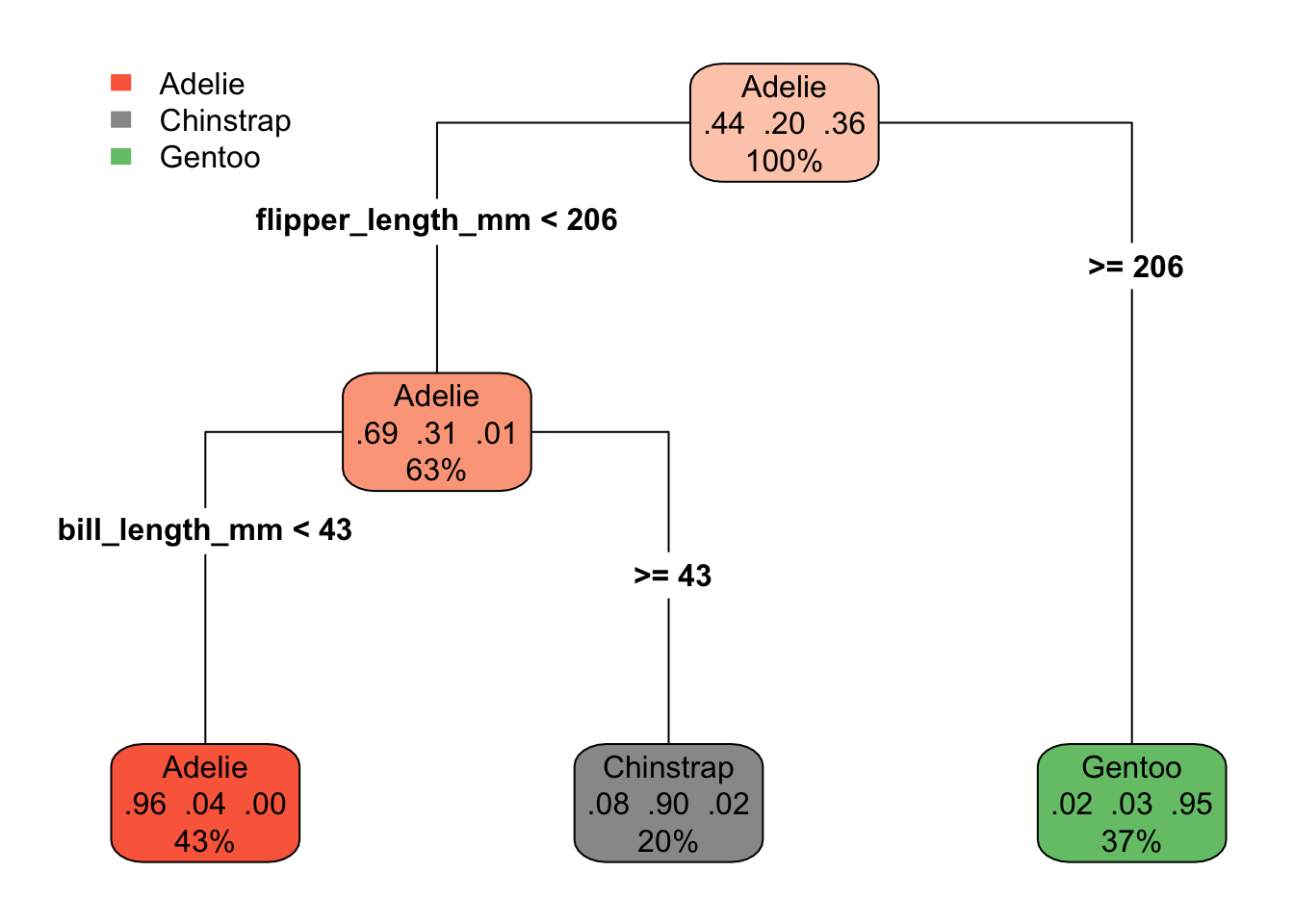
3. The Ensemble: Random Forest (“Colony of Agents”)
Many diverse trees + aggregation = emergence.
Show the Code
rf_spec <- rand_forest(trees = 500, mtry = tune()) |>
  set_mode("classification") |>
  set_engine("ranger", importance = "permutation", seed = 123)

rf_wf <- workflow() |>
  add_formula(species ~ .) |>
  add_model(rf_spec)

# Tune mtry for diversity (commented out for faster execution in class)
# cv_folds <- vfold_cv(train, v = 5)
#
# rf_res <- rf_wf |>
#   tune_grid(
#     resamples = cv_folds,
#     grid = crossing(mtry = c(2, 4, 6, 8)),
#     metrics = metric_set(accuracy)
#   )

# For reliable teaching, use a fixed reasonable mtry (or uncomment tuning)
# best_params <- select_best(rf_res, "accuracy")
# cat("Best mtry:", best_params$mtry, "\n")

best_mtry <- 4 # Good default for penguins data (~half the predictors)

rf_fit <- rf_wf |>
  finalize_workflow(list(mtry = best_mtry)) |>
  fit(train)

# Evaluate
rf_pred <- predict(rf_fit, test, type = "class")
rf_acc <- mean(rf_pred$.pred_class == test$species)
cat("Random Forest Accuracy:", round(rf_acc, 3), "\n")
Random Forest Accuracy: 1 Key Observation: The ensemble is almost always more accurate and stable.
4. Visualizing Diversity — The Source of Emergence
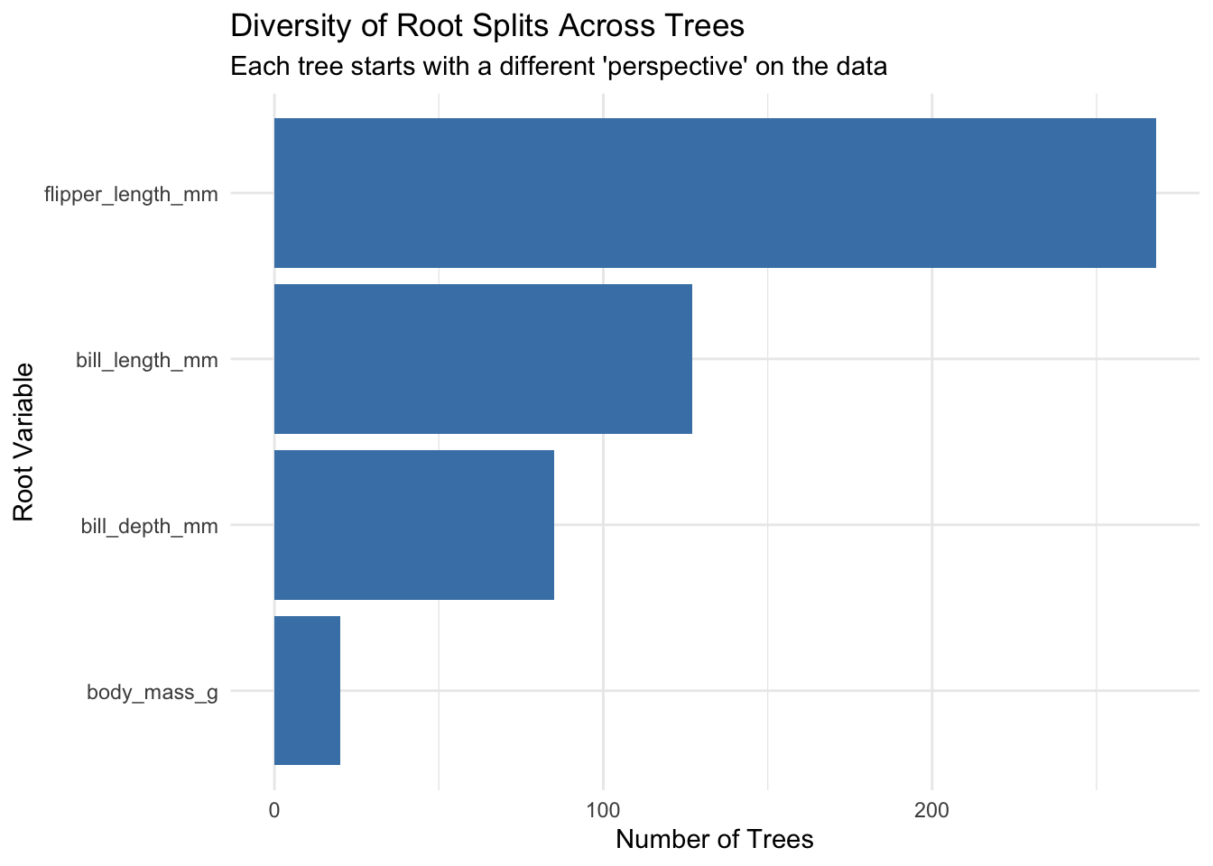
4.1 Root Split Diversity
Show the Code
extract_roots <- function(rf_model) {
  fit_obj <- extract_fit_engine(rf_model)
  map_chr(seq_len(fit_obj$num.trees), ~ ranger::treeInfo(fit_obj, tree = .x)$splitvarName[1])
}

roots <- extract_roots(rf_fit)
roots_df <- tibble(root_variable = roots) |>
  count(root_variable, sort = TRUE)

roots_df |>
  ggplot(aes(x = reorder(root_variable, n), y = n)) +
  geom_col(fill = "steelblue") +
  coord_flip() +
  labs(
    title = "Diversity of Root Splits Across Trees",
    subtitle = "Each tree starts with a different 'perspective' on the data",
    x = "Root Variable", y = "Number of Trees"
  )
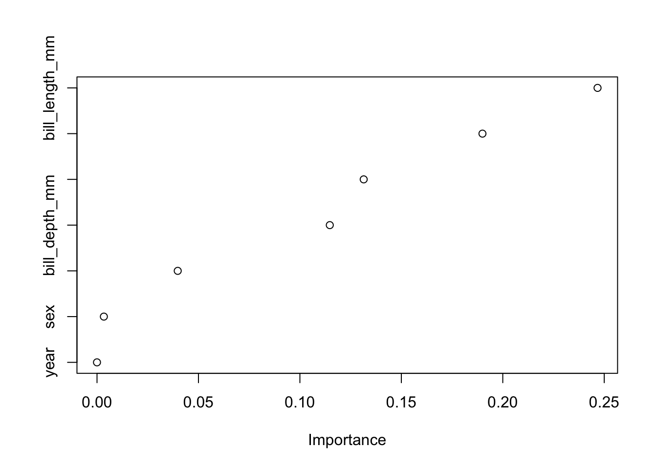
4.2 Collective Feature Importance
4.3 Single Tree vs Ensemble Decision Space (2D Projection)
Show the Code
# 2D subset for visualization
penguins_2d <- penguins |> select(bill_length_mm, bill_depth_mm, species)

# Simple single tree on 2 vars
tree_2d <- decision_tree() |>
  set_mode("classification") |>
  set_engine("rpart") |>
  fit(species ~ bill_length_mm + bill_depth_mm, data = train)

# RF on 2 vars
rf_2d_spec <- rand_forest(trees = 200) |>
  set_mode("classification") |>
  set_engine("ranger")

rf_2d_fit <- workflow(species ~ bill_length_mm + bill_depth_mm, rf_2d_spec) |>
  fit(train)

# Predictions grid for plotting (approximate boundaries)
grid <- expand.grid(
  bill_length_mm = seq(min(penguins$bill_length_mm), max(penguins$bill_length_mm), length.out = 100),
  bill_depth_mm = seq(min(penguins$bill_depth_mm), max(penguins$bill_depth_mm), length.out = 100)
)

grid_tree <- grid |>
  bind_cols(predict(tree_2d, grid, type = "class"))

grid_rf <- grid |>
  bind_cols(predict(rf_2d_fit, grid, type = "class"))

p1 <- ggplot() +
  geom_raster(data = grid_tree, aes(bill_length_mm, bill_depth_mm, fill = .pred_class), alpha = 0.35) +
  geom_point(data = penguins, aes(bill_length_mm, bill_depth_mm, color = species), alpha = 0.8) +
  labs(title = "Single Tree Decision Regions", subtitle = "Rigid, piecewise", fill = "Predicted", color = "Actual") +
  theme(legend.position = "none")

p2 <- ggplot() +
  geom_raster(data = grid_rf, aes(bill_length_mm, bill_depth_mm, fill = .pred_class), alpha = 0.35) +
  geom_point(data = penguins, aes(bill_length_mm, bill_depth_mm, color = species), alpha = 0.8) +
  labs(title = "Random Forest Decision Regions", subtitle = "Smoother, emergent from many trees", fill = "Predicted", color = "Actual")

p1 + p2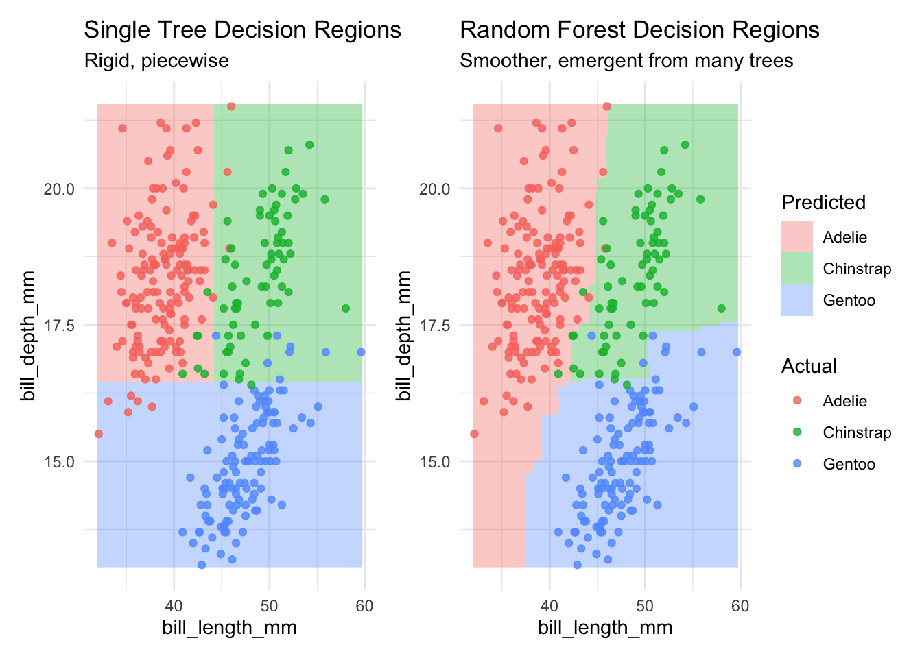
5. Complexity Science Analogies & Discussion
- Agents: Each tree is a simple agent making local greedy decisions on its bootstrap sample + random features.
- Local Rules: Greedy splitting based on information gain.
- Interactions & Aggregation: Bagging (parallel) + majority vote / averaging creates global coherence.
- Emergence: Robustness, better generalization, automatic feature interaction capture — properties not present in individual trees.
-
Compare to Nature:
- Ant colony optimization
- Bird flocking (boids)
- Neural networks (neurons as agents)
- Markets (traders as agents)
Prompt for students: How does changing mtry (feature randomness) affect diversity and performance? What does this teach us about “requisite variety” in complex systems?
6. Exercises
- Train a single tree and the RF. Compare confusion matrices using
conf_mat(). - Experiment with different numbers of trees and plot learning curves (accuracy vs. #trees).
- Extract 3 individual trees using
treeInfo()and compare their root splits. - Reflection essay (200 words): “In what ways do ensemble methods illustrate Philip Anderson’s ‘More is Different’?”
7. Extensions
-
Boosting: Replace with
boost_tree()+ LightGBM (bonsai). Sequential adaptation = adaptive agents. -
Agent-Based Simulation: Use
NetLogoRor custom loops to simulate simple “tree agents”. - Network View: Treat trees as nodes and shared splits as edges (using igraph).
Further Reading:
- Hands-On Machine Learning with R (tidymodels book)
- Complexity Science: Melanie Mitchell’s Complexity: A Guided Tour
- Original papers on Bagging (Breiman) and Boosting.