Logistic Regression
Logistic Regression with tidymodels — ISLR Default Dataset
Defaultis the classic textbook binary-classification dataset: 10,000 simulated credit-card customers, predicting whether each one defaults (Yes/No) from their student status, credit card balance, and income.
Packages needed: tidymodels, ISLR (for the Default data)
1. Load and inspect the data
data(Default, package = "ISLR")

default <- as_tibble(Default)

glimpse(default)
Rows: 10,000
Columns: 4
$ default <fct> No, No, No, No, No, No, No, No, No, No, No, No, No, No, No, No…
$ student <fct> No, Yes, No, No, No, Yes, No, Yes, No, No, Yes, Yes, No, No, N…
$ balance <dbl> 729.5265, 817.1804, 1073.5492, 529.2506, 785.6559, 919.5885, 8…
$ income <dbl> 44361.625, 12106.135, 31767.139, 35704.494, 38463.496, 7491.55…count(default, default) # note the class imbalance: ~3.3% default = "Yes"2. Split the data: train / test
set.seed(123)

default_split <- initial_split(default, prop = 0.80, strata = default)
default_train <- training(default_split)
default_test <- testing(default_split)
3. Preprocessing recipe
default_rec <-
  recipe(default ~ student + balance + income, data = default_train) |>
  step_dummy(all_nominal_predictors()) |>
  step_zv(all_predictors()) |>
  step_normalize(all_numeric_predictors())
4. Model specification
logreg_spec <-
  logistic_reg() |>
  set_engine("glm") |>
  set_mode("classification")
5. Workflow: bundle recipe + model
default_wflow <-
  workflow() |>
  add_recipe(default_rec) |>
  add_model(logreg_spec)
6. Fit on the training data
default_fit <- fit(default_wflow, data = default_train)

# Tidy view of coefficients (log-odds scale), sorted by magnitude
default_fit |>
  extract_fit_parsnip() |>
  tidy() |>
  arrange(desc(abs(estimate)))
7. Evaluate with 10-fold cross-validation (on training data)
set.seed(456)
default_folds <- vfold_cv(default_train, v = 10, strata = default)

# "Yes" is the event of interest but comes second alphabetically, so tell
# yardstick which level counts as the "event" for sensitivity/specificity
class_metrics <- metric_set(roc_auc, accuracy, sensitivity, specificity)

default_cv_results <-
  default_wflow |>
  fit_resamples(
    resamples = default_folds,
    metrics   = class_metrics,
    control   = control_resamples(save_pred = TRUE)
  )

collect_metrics(default_cv_results)
8. Final fit on full training set + evaluation on the held-out test set
final_fit <- last_fit(
  default_wflow,
  split   = default_split,
  metrics = class_metrics
)
# Test-set performance
collect_metrics(final_fit)
# Predictions (class + probabilities) on the test set
test_predictions <- collect_predictions(final_fit)
head(test_predictions)9. Confusion matrix and ROC curve
test_predictions |>
  conf_mat(truth = default, estimate = .pred_class)
Truth
Prediction No Yes
No 1923 50
Yes 8 19test_predictions |>
roc_curve(truth = default, .pred_Yes) |>
autoplot() +
labs(title = "ROC Curve — Predicting Credit Card Default")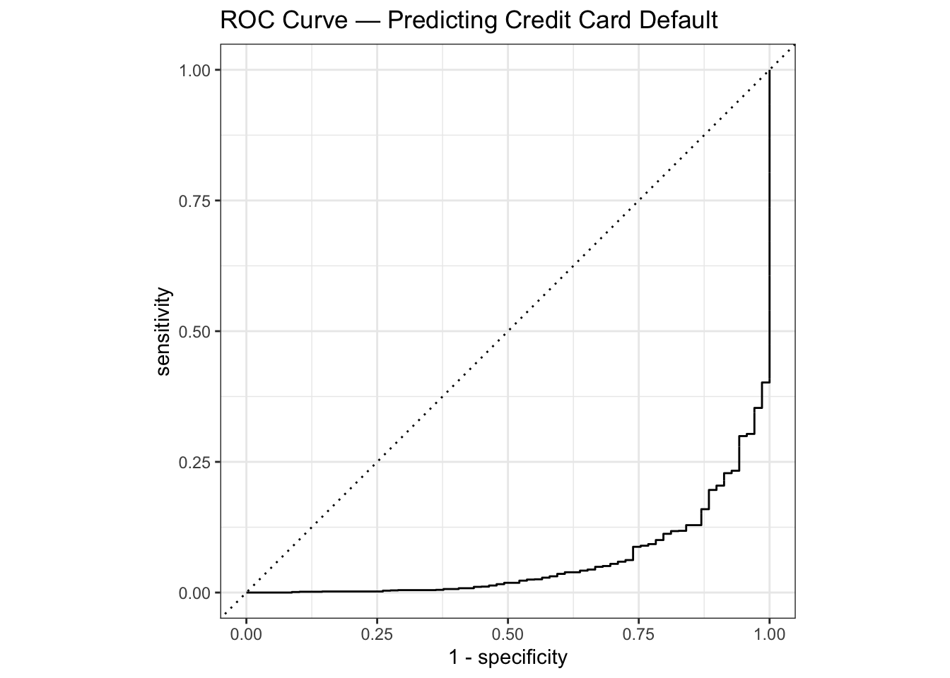
10. (Optional) Adjust the classification threshold
Because defaults are rare (~3.3%), the default 0.5 probability threshold will classify almost everyone as “No”. Lowering the threshold trades some precision for much better recall on the minority class.
11. (Optional) Extract the final fitted workflow for reuse / deployment
final_wflow_fit <- extract_workflow(final_fit)
# saveRDS(final_wflow_fit, "default_logreg_workflow.rds")

# Example: predict on new/unseen data using the finalized workflow
# predict(final_wflow_fit, new_data = some_new_data, type = "prob")