# install.packages("tidymodels")
# install.packages("kernlab")
# install.packages("titanic")

library(tidymodels)
library(titanic)
library(kernlab)
tidymodels_prefer()Support Vector Machines
Support Vector Machine Classification with tidymodels — Titanic Dataset
The full, labeled Titanic dataset (with the Survived outcome) is part of the titanic package as titanic::titanic_train.
Packages needed: tidymodels (includes kernlab via the “kernlab” engine):
1. Load and prepare the data
titanic_raw <- as_tibble(titanic_train)

titanic_df <- titanic_raw |>
  mutate(
    Survived = factor(
      if_else(Survived == 1, "yes", "no"),
      levels = c("yes", "no") # first level = the "event" of interest
    ),
    Pclass = factor(Pclass, levels = c(1, 2, 3), labels = c("1st", "2nd", "3rd")),
    Sex = factor(Sex),
    Embarked = na_if(Embarked, ""),
    Embarked = factor(Embarked)
  ) |>
  # Name, Ticket, and Cabin are high-cardinality free-text/ID fields that
  # need substantial feature engineering to be useful; PassengerId is just
  # a row identifier. All are dropped for this example.
  select(Survived, Pclass, Sex, Age, SibSp, Parch, Fare, Embarked)

glimpse(titanic_df)
Rows: 891
Columns: 8
$ Survived <fct> no, yes, yes, yes, no, no, no, no, yes, yes, yes, yes, no, no…
$ Pclass <fct> 3rd, 1st, 3rd, 1st, 3rd, 3rd, 1st, 3rd, 3rd, 2nd, 3rd, 1st, 3…
$ Sex <fct> male, female, female, female, male, male, male, male, female,…
$ Age <dbl> 22, 38, 26, 35, 35, NA, 54, 2, 27, 14, 4, 58, 20, 39, 14, 55,…
$ SibSp <int> 1, 1, 0, 1, 0, 0, 0, 3, 0, 1, 1, 0, 0, 1, 0, 0, 4, 0, 1, 0, 0…
$ Parch <int> 0, 0, 0, 0, 0, 0, 0, 1, 2, 0, 1, 0, 0, 5, 0, 0, 1, 0, 0, 0, 0…
$ Fare <dbl> 7.2500, 71.2833, 7.9250, 53.1000, 8.0500, 8.4583, 51.8625, 21…
$ Embarked <fct> S, C, S, S, S, Q, S, S, S, C, S, S, S, S, S, S, Q, S, S, C, S…count(titanic_df, Survived)Survived Pclass Sex Age SibSp Parch Fare Embarked
0 0 0 177 0 0 0 2 2. Split the data: train / test
set.seed(123)

titanic_split <- initial_split(titanic_df, prop = 0.80, strata = Survived)
titanic_train_set <- training(titanic_split)
titanic_test_set <- testing(titanic_split)
3. Preprocessing recipe
SVMs are distance-based, so — unlike the random forest example — scaling numeric predictors matters a lot here. We also need to impute missing values and dummy-code factors, since kernlab’s SVM implementation requires a fully numeric predictor matrix.
titanic_rec <-
  recipe(Survived ~ ., data = titanic_train_set) |>
  step_impute_median(Age, Fare) |>
  step_impute_mode(Embarked) |>
  step_dummy(all_nominal_predictors()) |>
  step_zv(all_predictors()) |>
  step_normalize(all_numeric_predictors())
4. Model specification (radial basis function kernel, tunable)
svm_spec <-
  svm_rbf(
    cost      = tune(),
    rbf_sigma = tune()
  ) |>
  set_engine("kernlab") |>
  set_mode("classification")
5. Workflow: bundle recipe + model
titanic_wflow <-
  workflow() |>
  add_recipe(titanic_rec) |>
  add_model(svm_spec)
6. Tune cost and rbf_sigma via cross-validation
set.seed(456)
titanic_folds <- vfold_cv(titanic_train_set, v = 10, strata = Survived)

class_metrics <- metric_set(roc_auc, accuracy, sensitivity, specificity)

set.seed(789)
svm_grid <- grid_regular(
  cost(range = c(-5, 5)), # log2 scale: 2^-5 to 2^5
  rbf_sigma(range = c(-5, 0)), # log10 scale: 1e-5 to 1
  levels = 5
)

svm_tune_results <-
  titanic_wflow |>
  tune_grid(
    resamples = titanic_folds,
    grid      = svm_grid,
    metrics   = class_metrics
  )
maximum number of iterations reached 0.009292639 -0.009257283maximum number of iterations reached 0.004636614 -0.004662125maximum number of iterations reached 0.009979506 -0.009934856maximum number of iterations reached 0.004640619 -0.004649566maximum number of iterations reached 0.01013137 -0.01008796maximum number of iterations reached 0.00522479 -0.005221429maximum number of iterations reached 0.009593184 -0.009555097maximum number of iterations reached 0.00465047 -0.004624215maximum number of iterations reached 0.009084122 -0.009052776maximum number of iterations reached 0.004670123 -0.004676457maximum number of iterations reached 0.00999773 -0.009954904maximum number of iterations reached 0.004669849 -0.00468095maximum number of iterations reached 0.009570994 -0.009533664maximum number of iterations reached 0.004506648 -0.004531009maximum number of iterations reached 0.00993294 -0.009891042maximum number of iterations reached 0.004869053 -0.004873603maximum number of iterations reached 0.009666797 -0.009626874maximum number of iterations reached 0.004480499 -0.004503718maximum number of iterations reached 0.01045123 -0.01040131maximum number of iterations reached 0.004641339 -0.004652208# Inspect the top-performing hyperparameter combinations by ROC AUC
show_best(svm_tune_results, metric = "roc_auc", n = 5)autoplot(svm_tune_results)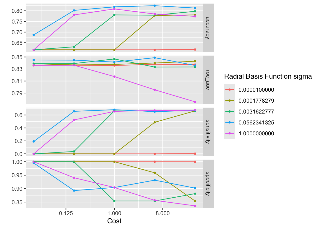
7. Select the best hyperparameters and finalize the workflow
best_svm <- select_best(svm_tune_results, metric = "roc_auc")

final_wflow <- finalize_workflow(titanic_wflow, best_svm)
8. Final fit on full training set + evaluation on the held-out test set
final_fit <- last_fit(
  final_wflow,
  split   = titanic_split,
  metrics = class_metrics
)

# Test-set performance
collect_metrics(final_fit)
# Predictions (class + probabilities) on the test set
test_predictions <- collect_predictions(final_fit)
head(test_predictions)9. Confusion matrix and ROC curve
test_predictions |>
  conf_mat(truth = Survived, estimate = .pred_class)
Truth
Prediction yes no
yes 51 6
no 18 104test_predictions |>
roc_curve(truth = Survived, .pred_yes) |>
autoplot() +
labs(title = "ROC Curve — Predicting Titanic Passenger Survival (SVM)")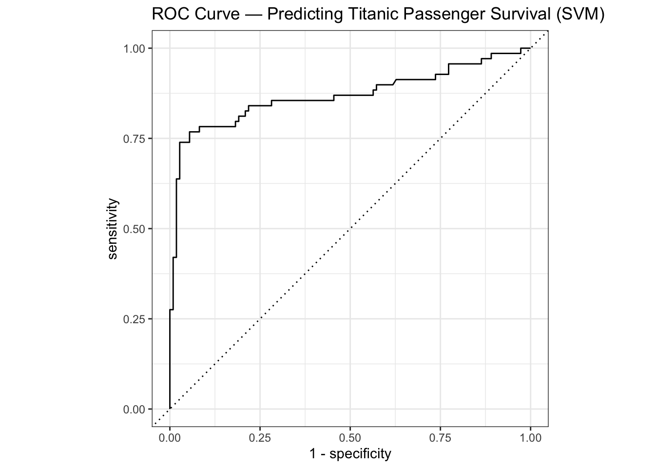
10. (Optional) Extract the final fitted workflow for reuse / deployment
final_wflow_fit <- extract_workflow(final_fit)
# saveRDS(final_wflow_fit, "titanic_svm_workflow.rds")

# Example: predict on new/unseen data using the finalized workflow
# predict(final_wflow_fit, new_data = some_new_data, type = "prob")